16.8: Теорема про розбіжність

Цілі навчання

• Поясніть значення теореми розбіжності.
• Використовуйте теорему розбіжності для обчислення потоку векторного поля.
• Застосуйте теорему розбіжності до електростатичного поля.

Розглянуто декілька версій фундаментальної теореми числення у вищих вимірах, які пов'язують інтеграл навколо орієнтованої межі області з «похідною» цієї сутності на орієнтованій області. У цьому розділі ми викладемо теорему розбіжності, яка є остаточною теоремою цього типу, яку ми будемо вивчати. Теорема розбіжності має багато застосувань у фізиці; зокрема, теорема розбіжності використовується в області рівнянь з частинними похідними для отримання рівнянь, що моделюють тепловий потік та збереження маси. Ми використовуємо теорему для обчислення інтегралів потоку та застосуємо її до електростатичних полів.

Огляд теорем

Перш ніж вивчати теорему розбіжності, корисно почати з огляду версій Фундаментальної теореми обчислення, про які ми обговорювали:

1. Фундаментальна теорема числення: $$\int_a^b f' (x) \, dx = f(b) - f(a). \nonumber$$ Ця теорема пов'язує інтеграл похідної$f'$ над відрізком прямої$[a,b]$ вздовж$x$ -осі з різницею$f$ оціненої на межі.
2. Фундаментальна теорема для лінійних інтегралів: $$\int_C \vecs \nabla f \cdot d\vecs r = f(P_1) - f(P_0), \nonumber$$ де$P_0$ початкова точка$C$ і$P_1$ є кінцевою точкою$C$. Фундаментальна теорема для лінійних інтегралів$C$ дозволяє шлях бути шлях у площині або в просторі, а не просто відрізок лінії на$x$ -осі. Якщо розглядати градієнт як похідну, то ця теорема пов'язує інтеграл похідної$\nabla f$ по шляху$C$ до різниці$f$ оцінюється на межі$C$.
3. Теорема Гріна, форма циркуляції: $$\iint_D (Q_x - P_y)\,dA = \int_C \vecs F \cdot d\vecs r. \nonumber$$ Оскільки$Q_x - P_y = \text{curl } \vecs F \cdot \mathbf{\hat k}$ і curl є похідною роду, теорема Гріна пов'язує інтеграл похідного завитка$\vecs F$ над$D$ плоскою областю з інтегралом$\vecs F$ над межею$D$.
4. Теорема Гріна, форма потоку: $$\iint_D (P_x + Q_y)\,dA = \int_C \vecs F \cdot \vecs N \, dS. \nonumber$$ Оскільки$P_x + Q_y = \text{div }\vecs F$ і дивергенція є похідною роду, форма потоку теореми Гріна пов'язує інтеграл похідної div$\vecs F$ над планарною$D$ областю з інтегралом$\vecs F$ над межею$D$.
5. Теорема Стокса: $$\iint_S curl \, \vecs F \cdot d\vecs S = \int_C \vecs F \cdot d\vecs r. \nonumber$$ Якщо розглядати завиток як похідну роду, то теорема Стокса пов'язує інтеграл похідного завитка$\vecs F$ над поверхнею$S$ (не обов'язково плоского) з інтегралом$\vecs F$ над межею$S$.

Постановка теореми про дивергенцію

Теорема про розбіжність слідує загальній закономірності цих інших теорем. Якщо розглядати дивергенцію як похідну роду, то теорема про дивергенцію пов'язує потрійний інтеграл похідної div$\vecs F$ над твердим тілом з інтегралом потоку$\vecs F$ над межею твердого тіла. Більш конкретно, теорема про розбіжність пов'язує інтеграл потоку векторного поля$\vecs F$ над замкнутою поверхнею$S$ з потрійним інтегралом розбіжності$\vecs F$ над тілом, укладеним$S$.

Теорема про розбіжність

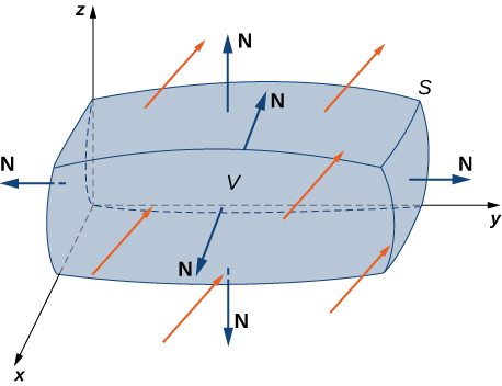
$S$Дозволяти бути кусково, гладка замкнута поверхня, яка охоплює тверде$E$ тіло в просторі. Припустимо,$S$ що орієнтований назовні, і$\vecs F$ нехай векторне поле з неперервними частинними похідними на відкритій області, що містить$E$ (рис.$\PageIndex{1}$). Тоді

$$\iiint_E \text{div }\vecs F \, dV = \iint_S \vecs F \cdot d\vecs S. \label{divtheorem}$$

Рисунок$\PageIndex{1}$: Теорема про розбіжність пов'язує інтеграл потоку через$S$ замкнуту поверхню з потрійним інтегралом над твердим$E$ тілом, укладеним поверхнею.

Нагадаємо, що форма потоку теореми Гріна стверджує, що

$$\iint_D \text{div }\vecs F \, dA = \int_C \vecs F \cdot \vecs N \, dS. \nonumber$$

Тому теорема розбіжності є версією теореми Гріна в одному вищому вимірі.

Доказ теореми про дивергенцію виходить за рамки цього тексту. Однак ми дивимося на неформальний доказ, який дає загальне уявлення про те, чому теорема вірна, але не доводить теорему з повною суворістю. Це пояснення слідує неформальному поясненню, чому теорема Стокса вірна.

Доказ

$B$Дозволяти бути невеликою коробкою зі сторонами, паралельними координатним площинам всередині$E$ (рис.$\PageIndex{2a}$). Нехай центр$B$ має координати$(x,y,z)$ і припустимо довжини країв$\Delta x, \, \Delta y$, і$\Delta z$. (Малюнок$\PageIndex{1b}$). Нормальний вектор з верхньої частини поля є$\mathbf{\hat k}$ і нормальний вектор з нижньої частини поля$-\mathbf{\hat k}$. Точковий добуток$\vecs F = \langle P, Q, R \rangle$ з$\mathbf{\hat k}$ є$R$ і крапковий добуток з$-\mathbf{\hat k}$ є$-R$. Площа верхньої частини коробки (і нижньої частини коробки)$\Delta S$ дорівнює$\Delta x \Delta y$.

Малюнок$\PageIndex{2}$: (а) Невелика коробка$B$ всередині поверхні$E$ має сторони, паралельні координатним площинам. (b) Коробка$B$ має довжину сторін$\Delta x, \, \Delta y$, і$\Delta z$ (c) Якщо ми подивимось на вигляд збоку$B$, ми бачимо, що, оскільки$(x,y,z)$ це центр коробки, щоб дістатися до верхньої частини коробки, ми повинні пройти вертикальну відстань$\Delta z$ вгору від$(x,y,z)$. Аналогічно, щоб дістатися до нижньої частини коробки, ми повинні пройти відстань$\Delta z$ вниз$(x,y,z)$.

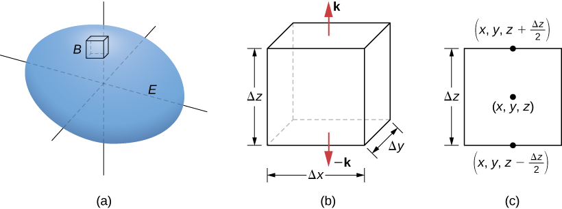
Флюс з верхньої частини коробки можна наблизити по$R \left(x,\, y,\, z + \frac{\Delta z}{2}\right) \,\Delta x \,\Delta y$ (рис.$\PageIndex{2c}$) і флюс з нижньої частини коробки є$- R \left(x,\, y,\, z - \frac{\Delta z}{2}\right) \,\Delta x \,\Delta y$. Якщо позначити різницю між цими значеннями як$\Delta R$, то чистий потік у вертикальному напрямку можна наблизити по$\Delta R\, \Delta x \,\Delta y$. Однак,

$$\Delta R \,\Delta x \,\Delta y = \left(\frac{\Delta R}{\Delta z}\right) \,\Delta x \,\Delta y \Delta z \approx \left(\frac{\partial R}{\partial z}\right) \,\Delta V.\nonumber$$

Тому чистий потік у вертикальному напрямку можна наблизити$\left(\frac{\partial R}{\partial z}\right)\Delta V$. Аналогічно, чистий потік в$x$ -напрямку може бути наближений$\left(\frac{\partial P}{\partial x}\right)\,\Delta V$ і чистий потік в$y$ -напрямку може бути наближений$\left(\frac{\partial Q}{\partial y}\right)\,\Delta V$. Додавання флюсів у всіх трьох напрямках дає наближення загального потоку з коробки:

$$\text{Total flux }\approx \left(\frac{\partial P}{\partial x} + \frac{\partial Q}{\partial y} + \frac{\partial R}{\partial z} \right) \Delta V = \text{div }\vecs F \,\Delta V. \nonumber$$

Це наближення стає довільно близьким до значення загального потоку, оскільки обсяг коробки зменшується до нуля.

Сума$\text{div }\vecs F \,\Delta V$ над усіма маленькими коробочками$E$ наближається приблизно$\iiint_E \text{div }\vecs F \,dV$. З іншого боку, сума$\text{div }\vecs F \,\Delta V$ над усіма маленькими коробками, що наближаються,$E$ - це сума потоків над усіма цими коробками. Так само, як і в неофіційному доведенні теореми Стокса, додавання цих потоків над усіма коробками призводить до скасування багатьох термінів. Якщо апроксимуюча коробка розділяє грань з іншою наближеною коробкою, то потік над однією гранню є негативом потоку над спільною гранню сусідньої коробки. Ці два інтеграли скасовують. При складанні всіх потоків єдиними інтегралами потоку, які виживають, є інтеграли над гранями, що наближаються до межі$E$. Оскільки обсяги наближених коробок зменшуються до нуля, це наближення стає довільно близьким до потоку над$S$.

$\Box$

Приклад$\PageIndex{1}$: Verifying the Divergence Theorem

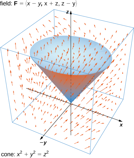
Перевірте теорему розбіжності для векторного поля$\vecs F = \langle x - y, \, x + z, \, z - y \rangle$ і поверхні,$S$ що складається з конуса$x^2 + y^2 = z^2, \, 0 \leq z \leq 1$, і кругової вершини конуса (див. Наступний малюнок). Припустимо, ця поверхня позитивно орієнтована.

Рішення

Нехай$E$ be the solid cone enclosed by $S$. To verify the theorem for this example, we show that

$$\iiint_E \text{div } \vecs F \,dV = \iint_S \vecs F \cdot d\vecs S\nonumber$$

by calculating each integral separately.

To compute the triple integral, note that $\text{div } \vecs F = P_x + Q_y + R_z = 2$, and therefore the triple integral is

$$\begin{align*} \iiint_E \text{div } \vecs F \, dV &= 2 \iiint_E dV \\[4pt] &= 2 \, (volume \, of \, E). \end{align*}$$

The volume of a right circular cone is given by $\pi r^2 \frac{h}{3}$. In this case, $h = r = 1$. Therefore,

$$\iiint_E \text{div } \vecs F \,dV = 2 \, (volume \, of \, E) = \frac{2\pi}{3}.\nonumber$$

To compute the flux integral, first note that $S$ is piecewise smooth; $S$ can be written as a union of smooth surfaces. Therefore, we break the flux integral into two pieces: one flux integral across the circular top of the cone and one flux integral across the remaining portion of the cone. Call the circular top $S_1$ and the portion under the top $S_2$. We start by calculating the flux across the circular top of the cone. Notice that $S_1$ has parameterization

$$\vecs r(u,v) = \langle u \, \cos v, \, u \, \sin v, \, 1 \rangle, \, 0 \leq u \leq 1, \, 0 \leq v \leq 2\pi.\nonumber$$

Then, the tangent vectors are $\vecs t_u = \langle \cos v, \, \sin v, \, 0 \rangle$ and $\vecs t_v = \langle -u \, \sin v, \, u \, \cos v, 0 \rangle$. Therefore, the flux across $S_1$ is

$$\begin{align*} \iint_{S_1} \vecs F \cdot d\vecs S &= \int_0^1 \int_0^{2\pi} \vecs F (\vecs r ( u,v)) \cdot (\vecs t_u \times \vecs t_v) \, dA \\[4pt] &= \int_0^1 \int_0^{2\pi} \langle u \, \cos v - u \, \sin v, \, u \, \cos v + 1, \, 1 - u \, \sin v \rangle \cdot \langle 0,0,u \rangle \, dv\, du \\[4pt] &= \int_0^1 \int_0^{2\pi} u - u^2 \sin v \, dv du \\[4pt] &= \pi. \end{align*}$$

We now calculate the flux over $S_2$. A parameterization of this surface is

$$\vecs r(u,v) = \langle u \, \cos v, \, u \, \sin v, \, u \rangle, \, 0 \leq u \leq 1, \, 0 \leq v \leq 2\pi.\nonumber$$

The tangent vectors are $\vecs t_u = \langle \cos v, \, \sin v, \, 1 \rangle$ and $\vecs t_v = \langle -u \, \sin v, \, u \, \cos v, 0 \rangle$, so the cross product is

$$\vecs t_u \times \vecs t_v = \langle - u \, \cos v, \, -u \, \sin v, \, u \rangle.\nonumber$$

Notice that the negative signs on the $x$ and $y$ components induce the negative (or inward) orientation of the cone. Since the surface is positively oriented, we use vector $\vecs t_v \times \vecs t_u = \langle u \, \cos v, \, u \, \sin v, \, -u \rangle$ in the flux integral. The flux across $S_2$ is then

$$\begin{align*} \iint_{S_2} \vecs F \cdot d\vecs S &= \int_0^1 \int_0^{2\pi} \vecs F ( \vecs r ( u,v)) \cdot (\vecs t_u \times \vecs t_v) \, dA \\[4pt] &= \int_0^1 \int_0^{2\pi} \langle u \, \cos v - u \, \sin v, \, u \, \cos v + u, \, u \, - u\sin v \rangle \cdot \langle u \, \cos v, \, u \, \sin v, \, -u \rangle\,dv\,du \\[4pt] &= \int_0^1 \int_0^{2\pi} u^2 \cos^2 v + 2u^2 \sin v - u^2 \,dv\,du \\[4pt] &= -\frac{\pi}{3} \end{align*}$$

The total flux across $S$ is

$$\iint_{S} \vecs F \cdot d\vecs S = \iint_{S_1}\vecs F \cdot d\vecs S + \iint_{S_2} \vecs F \cdot d\vecs S = \frac{2\pi}{3} = \iiint_E \text{div } \vecs F \,dV,\nonumber$$

and we have verified the divergence theorem for this example.

Exercise $\PageIndex{1}$

Verify the divergence theorem for vector field $\vecs F (x,y,z) = \langle x + y + z, \, y, \, 2x - y \rangle$ and surface $S$ given by the cylinder $x^2 + y^2 = 1, \, 0 \leq z \leq 3$ plus the circular top and bottom of the cylinder. Assume that $S$ is positively oriented.

Hint

Calculate both the flux integral and the triple integral with the divergence theorem and verify they are equal.

Answer

Both integrals equal $6\pi$.

​​Recall that the divergence of continuous field $\vecs F$ at point $P$ is a measure of the “outflowing-ness” of the field at $P$. If $\vecs F$ represents the velocity field of a fluid, then the divergence can be thought of as the rate per unit volume of the fluid flowing out less the rate per unit volume flowing in. The divergence theorem confirms this interpretation. To see this, let $P$ be a point and let $B_{\tau}$ be a ball of small radius $r$ centered at $P$ (Figure $\PageIndex{3}$). Let $S_{\tau}$ be the boundary sphere of $B_{\tau}$. Since the radius is small and $\vecs F$ is continuous, $\text{div }\vecs F(Q) \approx \text{div }\vecs F(P)$ for all other points $Q$ in the ball. Therefore, the flux across $S_{\tau}$ can be approximated using the divergence theorem:

$$\iint_{S_{\tau}} \vecs F \cdot d\vecs S = \iiint_{B_{\tau}} \text{div }\vecs F \,dV \approx \iiint_{B_{\tau}} \text{div }\vecs F(P) \,dV.\nonumber$$

Since $div F(P)$ is a constant,

$$\iiint_{B_{\tau}} \text{div }\vecs F(P) \,dV = \text{div }\vecs F(P) \, V(B_{\tau}).\nonumber$$

Therefore, flux $$\iint_{S_{\tau}} \vecs F \cdot d\vecs S \nonumber$$ can be approximated by $\vecs F(P) \, V(B_{\tau})$. This approximation gets better as the radius shrinks to zero, and therefore

$$\text{div } \vecs F(P) = \lim_{\tau \rightarrow 0} \frac{1}{V(B_{\tau})} \iint_{S_{\tau}} \vecs F \cdot d\vecs S.\nonumber$$

This equation says that the divergence at $P$ is the net rate of outward flux of the fluid per unit volume.

Figure $\PageIndex{3}$: Ball $B_{\tau}$ of small radius $r$ centered at $P$.

Using the Divergence Theorem

The divergence theorem translates between the flux integral of closed surface $S$ and a triple integral over the solid enclosed by $S$. Therefore, the theorem allows us to compute flux integrals or triple integrals that would ordinarily be difficult to compute by translating the flux integral into a triple integral and vice versa.

Example $\PageIndex{2}$: Applying the Divergence Theorem

Calculate the surface integral

$$\iint_S \vecs F \cdot d\vecs S, \nonumber$$

where $S$ is cylinder $x^2 + y^2 = 1, \, 0 \leq z \leq 2$, including the circular top and bottom, and $\vecs F = \left\langle \frac{x^3}{3} + yz, \, \frac{y^3}{3} - \sin (xz), \, z - x - y \right\rangle$.

Solution

We could calculate this integral without the divergence theorem, but the calculation is not straightforward because we would have to break the flux integral into three separate integrals: one for the top of the cylinder, one for the bottom, and one for the side. Furthermore, each integral would require parameterizing the corresponding surface, calculating tangent vectors and their cross product..

By contrast, the divergence theorem allows us to calculate the single triple integral

$$\iiint_E \text{div }\vecs F \, dV,\nonumber$$

where $E$ is the solid enclosed by the cylinder. Using the divergence theorem (Equation $\ref{divtheorem}$) and converting to cylindrical coordinates, we have

$$\begin{align*} \iint_S \vecs F \cdot d\vecs S &= \iiint_E \text{div }\vecs F \, dV, \\[4pt] &= \iiint_E (x^2 + y^2 + 1) \, dV \\[4pt] &= \int_0^{2\pi} \int_0^1 \int_0^2 (r^2 + 1) \, r \, dz \, dr \, d\theta \\[4pt] &= \frac{3}{2} \int_0^{2\pi} d\theta \\[4pt] &= 3\pi. \end{align*}$$

Exercise $\PageIndex{2}$

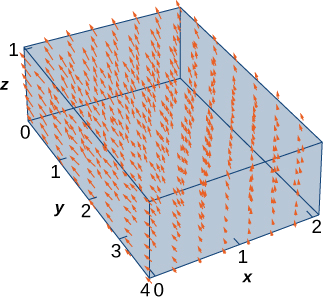
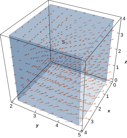
Use the divergence theorem to calculate flux integral $$\iint_S \vecs F \cdot d\vecs S,\nonumber$$ where $S$ is the boundary of the box given by $0 \leq x \leq 2, \, 0 \leq y \leq 4, \, 0 \leq z \leq 1$ and $\vecs F = \langle x^2 + yz, \, y - z, \, 2x + 2y + 2z \rangle$ (see the following figure).

Підказка

Обчисліть відповідний потрійний інтеграл.

Відповідь

40

Приклад$\PageIndex{3}$: Applying the Divergence Theorem

$\vecs v = \left\langle - \frac{y}{z}, \, \frac{x}{z}, \, 0 \right\rangle$Дозволяти бути поле швидкості рідини. $C$Дозволяти твердий куб$1 \leq x \leq 4, \, 2 \leq y \leq 5, \, 1 \leq z \leq 4$, заданий, і$S$ нехай межа цього куба (див. Наступний малюнок). Знайдіть швидкість потоку рідини поперек$S$.

Малюнок$\PageIndex{4}$: Векторне поле$\vecs v = \left\langle - \frac{y}{z}, \, \frac{x}{z}, \, 0 \right\rangle$.

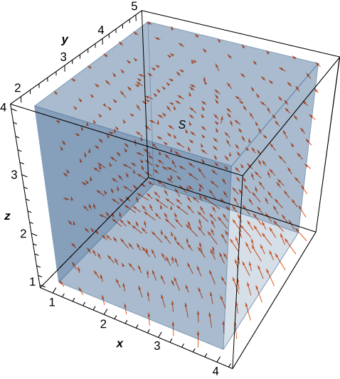
Рішення

Витрата рідини поперек$S$ становить$\iint_S \vecs v \cdot d\vecs S$. Перш ніж обчислити цей інтеграл потоку, давайте обговоримо, яким має бути значення інтеграла. Виходячи з малюнка$\PageIndex{4}$, ми бачимо, що якщо ми помістимо цей куб у рідину (до тих пір, поки куб не охоплює походження), то швидкість потрапляння рідини в куб така ж, як швидкість виходу рідини з куба. Поле має обертальний характер, і для даного кола паралельно$xy$ -площині, яка має центр на осі z, вектори вздовж цього кола мають однакову величину. Ось як ми можемо бачити, що швидкість потоку однакова, що входить і виходить з куба. Потік в куб скасовується при витіканні з куба, і тому витрата рідини через куб повинна дорівнювати нулю.

Щоб переконатися в цій інтуїції, нам потрібно обчислити інтеграл потоку. Розрахунок інтеграла потоку безпосередньо вимагає розбиття інтеграла потоку на шість окремих інтегралів потоку, по одному для кожної грані куба. Нам також потрібно знайти дотичні вектори, обчислити їх перехресний добуток. Однак використання теореми розбіжності робить цей розрахунок набагато швидше:

\ [\ почати {вирівнювати*}\ iInt_s\ vecs v\ cdot d\ vecs S &=\ IIint_c\ текст {div}\ vecs v\, dV\\ [4pt]
&=\ IIint_c 0\, dV = 0. \ end {вирівнювати*}\]

Тому потік дорівнює нулю, як і очікувалося.

Вправа$\PageIndex{3}$

$\vecs v = \left\langle \frac{x}{z}, \, \frac{y}{z}, \, 0 \right\rangle$Дозволяти бути поле швидкості рідини. $C$Дозволяти твердий куб$1 \leq x \leq 4, \, 2 \leq y \leq 5, \, 1 \leq z \leq 4$, заданий, і$S$ нехай межа цього куба (див. Наступний малюнок). Знайдіть швидкість потоку рідини поперек$S$.

Підказка

Скористайтеся теоремою розбіжності та обчисліть потрійний інтеграл

Відповідь

$9 \, \ln (16)$

Example illustrates a remarkable consequence of the divergence theorem. Let $S$ be a piecewise, smooth closed surface and let $\vecs F$ be a vector field defined on an open region containing the surface enclosed by $S$. If $\vecs F$ has the form $F = \langle f (y,z), \, g(x,z), \, h(x,y)\rangle$, then the divergence of $\vecs F$ is zero. By the divergence theorem, the flux of $\vecs F$ across $S$ is also zero. This makes certain flux integrals incredibly easy to calculate. For example, suppose we wanted to calculate the flux integral $\iint_S \vecs F \cdot d\vecs S$ where $S$ is a cube and

$$\vecs F = \langle \sin (y) \, e^{yz}, \, x^2z^2, \, \cos (xy) \, e^{\sin x} \rangle. \nonumber$$

Calculating the flux integral directly would be difficult, if not impossible, using techniques we studied previously. At the very least, we would have to break the flux integral into six integrals, one for each face of the cube. But, because the divergence of this field is zero, the divergence theorem immediately shows that the flux integral is zero.

We can now use the divergence theorem to justify the physical interpretation of divergence that we discussed earlier. Recall that if $\vecs F$ is a continuous three-dimensional vector field and $P$ is a point in the domain of $\vecs F$, then the divergence of $\vecs F$ at $P$ is a measure of the “outflowing-ness” of $\vecs F$ at $P$. If $\vecs F$ represents the velocity field of a fluid, then the divergence of $\vecs F$ at $P$ is a measure of the net flow rate out of point $P$ (the flow of fluid out of $P$ less the flow of fluid in to $P$). To see how the divergence theorem justifies this interpretation, let $B_{\tau}$ be a ball of very small radius r with center $P$, and assume that $B_{\tau}$ is in the domain of $\vecs F$. Furthermore, assume that $B_{\tau}$ has a positive, outward orientation. Since the radius of $B_{\tau}$ is small and $\vecs F$ is continuous, the divergence of $\vecs F$ is approximately constant on $B_{\tau}$. That is, ifv $P'$ is any point in $B_{\tau}$, then $\text{div } \vecs F(P) \approx \text{div } \vecs F(P')$. Let $S_{\tau}$ denote the boundary sphere of $B_{\tau}$. We can approximate the flux across $S_{\tau}$ using the divergence theorem as follows:

$$\begin{align*} \iint_{S_{\tau}} \vecs F \cdot d\vecs S &= \iiint_{B_{\tau}} \text{div }\vecs F \, dV \\[4pt] &\approx \iiint_{B_{\tau}} \text{div } \vecs F (P) \, dV \\[4pt] &= \text{div } \vecs F (P) \, V(B_{\tau}). \end{align*}$$

As we shrink the radius $r$ to zero via a limit, the quantity $\text{div }\vecs F (P) \, V(B_{\tau})$ gets arbitrarily close to the flux. Therefore,

$$\text{div }\vecs F(P) = \lim_{\tau \rightarrow 0} \frac{1}{V(B_{\tau})} \iint_{S_{\tau}} \vecs F \cdot d\vecs S \nonumber$$

and we can consider the divergence at $P$ as measuring the net rate of outward flux per unit volume at $P$. Since “outflowing-ness” is an informal term for the net rate of outward flux per unit volume, we have justified the physical interpretation of divergence we discussed earlier, and we have used the divergence theorem to give this justification.

Application to Electrostatic Fields

The divergence theorem has many applications in physics and engineering. It allows us to write many physical laws in both an integral form and a differential form (in much the same way that Stokes’ theorem allowed us to translate between an integral and differential form of Faraday’s law). Areas of study such as fluid dynamics, electromagnetism, and quantum mechanics have equations that describe the conservation of mass, momentum, or energy, and the divergence theorem allows us to give these equations in both integral and differential forms.

One of the most common applications of the divergence theorem is to electrostatic fields. An important result in this subject is Gauss’ law. This law states that if $S$ is a closed surface in electrostatic field $\vecs E$, then the flux of $\vecs E$ across $S$ is the total charge enclosed by $S$ (divided by an electric constant). We now use the divergence theorem to justify the special case of this law in which the electrostatic field is generated by a stationary point charge at the origin.

If $(x,y,z)$ is a point in space, then the distance from the point to the origin is $r = \sqrt{x^2 + y^2 + z^2}$. Let $\vecs F_{\tau}$ denote radial vector field $\vecs F_{\tau} = \dfrac{1}{\tau^2} \left\langle \dfrac{x}{\tau}, \, \dfrac{y}{\tau}, \, \dfrac{z}{\tau}\right\rangle$.The vector at a given position in space points in the direction of unit radial vector $\left\langle \dfrac{x}{\tau}, \, \dfrac{y}{\tau}, \, \dfrac{z}{\tau}\right\rangle$ and is scaled by the quantity $1/\tau^2$. Therefore, the magnitude of a vector at a given point is inversely proportional to the square of the vector’s distance from the origin. Suppose we have a stationary charge of $q$ Coulombs at the origin, existing in a vacuum. The charge generates electrostatic field $\vecs E$ given by

$$\vecs E = \dfrac{q}{4\pi \epsilon_0}\vecs F_{\tau}, \nonumber$$

where the approximation $\epsilon_0 = 8.854 \times 10^{-12}$ farad (F)/m is an electric constant. (The constant $\epsilon_0$ is a measure of the resistance encountered when forming an electric field in a vacuum.) Notice that $\vecs E$ is a radial vector field similar to the gravitational field described in [link]. The difference is that this field points outward whereas the gravitational field points inward. Because

$$\vecs E = \dfrac{q}{4\pi \epsilon_0}\vecs F_{\tau} = \dfrac{q}{4\pi \epsilon_0}\left(\dfrac{1}{\tau^2} \left\langle \dfrac{x}{\tau}, \, \dfrac{y}{\tau}, \, \dfrac{z}{\tau}\right\rangle\right), \nonumber$$

we say that electrostatic fields obey an inverse-square law. That is, the electrostatic force at a given point is inversely proportional to the square of the distance from the source of the charge (which in this case is at the origin). Given this vector field, we show that the flux across closed surface $S$ is zero if the charge is outside of $S$, and that the flux is $q/epsilon_0$ if the charge is inside of $S$. In other words, the flux across S is the charge inside the surface divided by constant $\epsilon_0$. This is a special case of Gauss’ law, and here we use the divergence theorem to justify this special case.

To show that the flux across $S$ is the charge inside the surface divided by constant $\epsilon_0$, we need two intermediate steps. First we show that the divergence of $\vecs F_{\tau}$ is zero and then we show that the flux of $\vecs F_{\tau}$ across any smooth surface $S$ is either zero or $4\pi$. We can then justify this special case of Gauss’ law.

Example $\PageIndex{4}$: The Divergence of $F_{\tau}$ is Zero

Verify that the divergence of $\vecs F_{\tau}$ is zero where $\vecs F_{\tau}$ is defined (away from the origin).

Solution

Since $\tau = \sqrt{x^2 + y^2 + z^2}$, the quotient rule gives us

$$\begin{align*} \dfrac{\partial}{\partial x} \left( \dfrac{x}{\tau^3} \right) &= \dfrac{\partial}{\partial x} \left( \dfrac{x}{(x^2+y^2+z^2)^{3/2}} \right) \\[4pt] &= \dfrac{(x^2+y^2+z^2)^{3/2} - x\left[\dfrac{3}{2} (x^2+y^2+z^2)^{1/2}2x\right]}{(x^2+y^2+z^2)^3} \\[4pt] &= \dfrac{\tau^3 -3x^2\tau}{\tau^6} = \dfrac{\tau^2 - 3x^2}{\tau^5}. \end{align*}$$

Similarly,

$$\dfrac{\partial}{\partial y} \left( \dfrac{y}{\tau^3} \right) = \dfrac{\tau^2 - 3y^2}{\tau^5} \, and \, \dfrac{\partial}{\partial z} \left( \dfrac{z}{\tau^3} \right) = \dfrac{\tau^2 - 3z^2}{\tau^5}. \nonumber$$

Therefore,

$$\begin{align*} \text{div } \vecs F_{\tau} &= \dfrac{\tau^2 - 3x^2}{\tau^5} + \dfrac{\tau^2 - 3y^2}{\tau^5} + \dfrac{\tau^2 - 3z^2}{\tau^5} \\[4pt] &= \dfrac{3\tau^2 - 3(x^2+y^2+z^2)}{\tau^5} \\[4pt] &= \dfrac{3\tau^2 - 3\tau^2}{\tau^5} = 0. \end{align*}$$

Notice that since the divergence of $\vecs F_{\tau}$ is zero and $\vecs E$ is $\vecs F_{\tau}$ scaled by a constant, the divergence of electrostatic field $\vecs E$ is also zero (except at the origin).

Flux across a Smooth Surface

Let $S$ be a connected, piecewise smooth closed surface and let $\vecs F_{\tau} = \dfrac{1}{\tau^2} \left\langle \dfrac{x}{\tau}, \, \dfrac{y}{\tau}, \, \dfrac{z}{\tau}\right \rangle$. Then,

$$\iint_S \vecs F_{\tau} \cdot d\vecs S = \begin{cases}0, & \text{if }S\text{ does not encompass the origin} \\ 4\pi, & \text{if }S\text{ encompasses the origin.} \end{cases} \nonumber$$

In other words, this theorem says that the flux of $\vecs F_{\tau}$ across any piecewise smooth closed surface $S$ depends only on whether the origin is inside of $S$.

Proof

The logic of this proof follows the logic of [link], only we use the divergence theorem rather than Green’s theorem.

First, suppose that $S$ does not encompass the origin. In this case, the solid enclosed by $S$ is in the domain of $\vecs F_{\tau}$, and since the divergence of $\vecs F_{\tau}$ is zero, we can immediately apply the divergence theorem and find that $$\iint_S \vecs F \cdot d\vecs S \nonumber$$ is zero.

Now suppose that $S$ does encompass the origin. We cannot just use the divergence theorem to calculate the flux, because the field is not defined at the origin. Let $S_a$ be a sphere of radius a inside of $S$ centered at the origin. The outward normal vector field on the sphere, in spherical coordinates, is

$$\vecs t_{\phi} \times \vecs t_{\theta} = \langle a^2 \cos \theta \, \sin^2 \phi, \, a^2 \sin \theta \, \sin^2 \phi, \, a^2 \sin \phi \, \cos \phi \rangle \nonumber$$

(see [link]). Therefore, on the surface of the sphere, the dot product $\vecs F_{\tau} \cdot \vecs N$ (in spherical coordinates) is

$$\begin{align*} \vecs F_{\tau} \cdot \vecs N &= \left \langle \dfrac{\sin \phi \, \cos \theta}{a^2}, \, \dfrac{\sin \phi \, \sin \theta}{a^2}, \, \dfrac{\cos \phi}{a^2} \right \rangle \cdot \langle a^2 \cos \theta \, \sin^2 \phi, a^2 \sin \theta \, \sin^2 \phi, \, a^2 \sin \phi \, \cos \phi \rangle \\[4pt] &= \sin \phi ( \langle \sin \phi \, \cos \theta, \, \sin \phi \, \sin \theta, \, \cos \phi \rangle \cdot \langle \sin \phi \, \cos \theta, \sin \phi \, \sin \theta, \, \cos \phi \rangle ) \\[4pt] &= \sin \phi. \end{align*}$$

The flux of $\vecs F_{\tau}$ across $S_a$ is

$$\iint_{S_a} \vecs F_{\tau} \cdot \vecs N dS = \int_0^{2\pi} \int_0^{\pi} \sin \phi \, d\phi \, d\theta = 4\pi. \nonumber$$

Now, remember that we are interested in the flux across $S$, not necessarily the flux across $S_a$. To calculate the flux across $S$, let $E$ be the solid between surfaces $S_a$ and $S$. Then, the boundary of $E$ consists of $S_a$ and $S$. Denote this boundary by $S - S_a$ to indicate that $S$ is oriented outward but now $S_a$ is oriented inward. We would like to apply the divergence theorem to solid $E$. Notice that the divergence theorem, as stated, can’t handle a solid such as $E$ because $E$ has a hole. However, the divergence theorem can be extended to handle solids with holes, just as Green’s theorem can be extended to handle regions with holes. This allows us to use the divergence theorem in the following way. By the divergence theorem,

$$\begin{align*} \iint_{S-S_a} \vecs F_{\tau} \cdot d\vecs S &= \iint_S \vecs F_{\tau} \cdot d\vecs S - \iint_{S_a} \vecs F_{\tau} \cdot d\vecs S \\[4pt] &= \iiint_E \text{div } \vecs F_{\tau} \, dV \\[4pt] &= \iiint_E 0 \, dV = 0. \end{align*}$$

Therefore,

$$\iint_S \vecs F_{\tau} \cdot d\vecs S = \iint_{S_a} \vecs F_{\tau} \cdot d\vecs S = 4\pi, \nonumber$$

and we have our desired result.

$\Box$

Now we return to calculating the flux across a smooth surface in the context of electrostatic field $\vecs E = \dfrac{q}{4\pi \epsilon_0} \vecs F_{\tau}$ of a point charge at the origin. Let $S$ be a piecewise smooth closed surface that encompasses the origin. Then

$$\begin{align*} \iint_S \vecs E \cdot d\vecs S &= \iint_S \dfrac{q}{4\pi \epsilon_0} \vecs F_{\tau} \cdot d\vecs S\\[4pt] &= \dfrac{q}{4\pi \epsilon_0} \iint_S \vecs F_{\tau} \cdot d\vecs S \\[4pt] &= \dfrac{q}{\epsilon_0}. \end{align*}$$

If $S$ does not encompass the origin, then

$$\iint_S \vecs E \cdot d\vecs S = \dfrac{q}{4\pi \epsilon_0} \iint_S \vecs F_{\tau} \cdot d\vecs S = 0. \nonumber$$

Therefore, we have justified the claim that we set out to justify: the flux across closed surface $S$ is zero if the charge is outside of $S$, and the flux is $q/\epsilon_0$ if the charge is inside of $S$.

This analysis works only if there is a single point charge at the origin. In this case, Gauss’ law says that the flux of $\vecs E$ across $S$ is the total charge enclosed by $S$. Gauss’ law can be extended to handle multiple charged solids in space, not just a single point charge at the origin. The logic is similar to the previous analysis, but beyond the scope of this text. In full generality, Gauss’ law states that if $S$ is a piecewise smooth closed surface and $Q$ is the total amount of charge inside of $S$, then the flux of $\vecs E$ across $S$ is $Q/\epsilon_0$.

Example $\PageIndex{5}$: Using Gauss’ law

Suppose we have four stationary point charges in space, all with a charge of 0.002 Coulombs (C). The charges are located at $(0,0,1), \, (1,1,4), (-1,0,0)$, and $(-2,-2,2)$. Let $\vecs E$ denote the electrostatic field generated by these point charges. If $S$ is the sphere of radius $2$ oriented outward and centered at the origin, then find

$$\iint_S \vecs E \cdot d\vecs S. \nonumber$$

Solution

According to Gauss’ law, the flux of $\vecs E$ across $S$ is the total charge inside of $S$ divided by the electric constant. Since $S$ has radius $2$, notice that only two of the charges are inside of $S$: the charge at $0,1,1)$ and the charge at $(-1,0,0)$. Therefore, the total charge encompassed by $S$ is $0.004$ and, by Gauss’ law,

$$\iint_S \vecs E \cdot d\vecs S = \dfrac{0.004}{8.854 \times 10^{-12}} \approx 4.418 \times 10^9 \, V - m. \nonumber$$

Exercise $\PageIndex{4}$

Work the previous example for surface $S$ that is a sphere of radius 4 centered at the origin, oriented outward.

Hint

Use Gauss’ law.

Answer

$\approx 6.777 \times 10^9$

Key Concepts

• The divergence theorem relates a surface integral across closed surface $S$ to a triple integral over the solid enclosed by $S$. The divergence theorem is a higher dimensional version of the flux form of Green’s theorem, and is therefore a higher dimensional version of the Fundamental Theorem of Calculus.
• The divergence theorem can be used to transform a difficult flux integral into an easier triple integral and vice versa.
• The divergence theorem can be used to derive Gauss’ law, a fundamental law in electrostatics.

Key Equations

• Divergence theorem $$\iiint_E \text{div } \vecs F \, dV = \iint_S \vecs F \cdot d\vecs S \nonumber$$

Glossary

divergence theorem

a theorem used to transform a difficult flux integral into an easier triple integral and vice versa

Gauss’ law

if S is a piecewise, smooth closed surface in a vacuum and $Q$ is the total stationary charge inside of $S$, then the flux of electrostatic field $\vecs E$ across $S$ is $Q/\epsilon_0$

inverse-square law

the electrostatic force at a given point is inversely proportional to the square of the distance from the source of the charge