6.2: Ортогональні доповнення

$\usepackage{macros} \newcommand{\lt}{<} \newcommand{\gt}{>} \newcommand{\amp}{&}$

Цілі навчання

1. Зрозумійте основні властивості ортогональних доповнень.
2. Навчіться обчислювати ортогональне доповнення підпростору.
3. Рецепти: ярлики для обчислення ортогональних доповнень загальних підпросторів.
4. Малюнок: ортогональні доповнення в$\mathbb{R}^2$ і$\mathbb{R}^3$.
5. Теорема: рядок рядка дорівнює рангу стовпця.
6. Словникові слова: ортогональне доповнення, пробіл рядків.

Важливо буде обчислити множину всіх векторів, які є ортогональними до заданого набору векторів. Виявляється, що вектор ортогональний набору векторів тоді і тільки тоді, коли він ортогональний до прольоту цих векторів, який є підпростором, тому ми обмежуємося випадком підпросторів.

Визначення ортогонального доповнення

Прийняття ортогонального доповнення - це операція, яка виконується на підпросторах.

Визначення$\PageIndex{1}$: Orthogonal Complement

$W$Дозволяти бути підпростором$\mathbb{R}^n$. Його ортогональним доповненням є підпростір

$$W^\perp = \bigl\{ \text{$v$ in $\mathbb{R}^n $}\mid v\cdot w=0 \text{ for all $w$ in $W$} \bigr\}. \nonumber$$

Символ іноді$W^\perp$ читається «$W$підступник».

Це набір усіх векторів$v$$\mathbb{R}^n$, які є ортогональними до всіх векторів в$W$. Нижче ми покажемо 15, що дійсно$W^\perp$ є підпростором.

Примітка$\PageIndex{1}$

Тепер у нас є два схожих на вигляд фрагменти позначення:

$$\begin{split} A^{\color{Red}T} \amp\text{ is the transpose of a matrix $A$}. \\ W^{\color{Red}\perp} \amp\text{ is the orthogonal complement of a subspace $W$}. \end{split} \nonumber$$

Намагайтеся не плутати ці два.

Картинки ортогональних доповнень

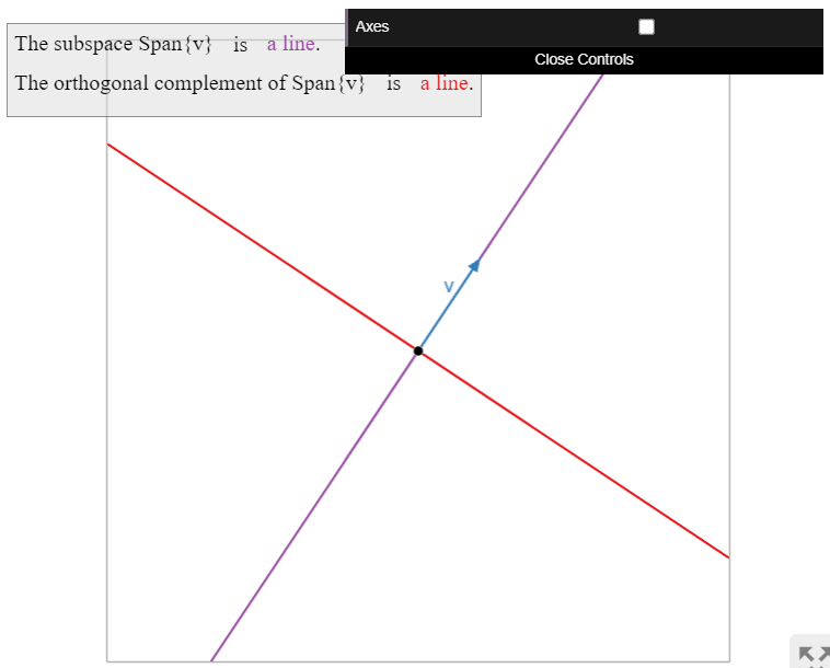
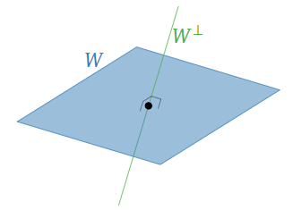
Ортогональне доповнення лінії$\color{blue}W$ через початок в$\mathbb{R}^2$ є перпендикулярною лінією$\color{Green}W^\perp$.

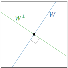
Малюнок$\PageIndex{1}$

Приклад$\PageIndex{1}$: Interactive: Orthogonal complements in $\mathbb{R}^2$

Малюнок$\PageIndex{2}$: The orthogonal complement of the line spanned by $v$ is the perpendicular line. Click and drag the head of $v$ to move it.

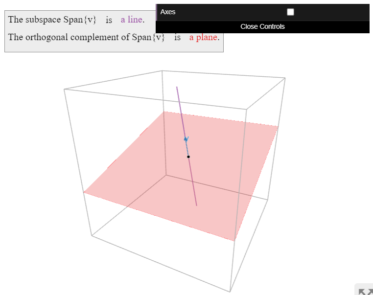
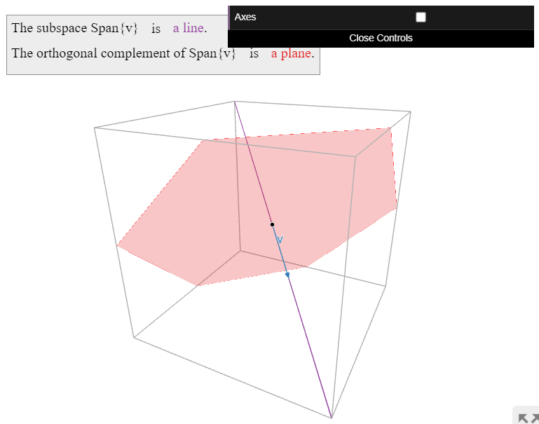
The orthogonal complement of a line $\color{blue}W$ in $\mathbb{R}^3$ is the perpendicular plane $\color{Green}W^\perp$.

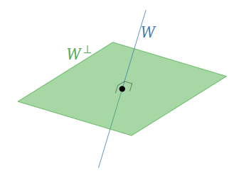
Figure $\PageIndex{3}$

Example $\PageIndex{2}$: Interactive: Orthogonal complements in $\mathbb{R}^3$

$\PageIndex{4}$:Малюнок Ортогональне доповнення лінії, що охоплюється,$v$ є перпендикулярною площиною. Клацніть і перетягніть голову$v$, щоб перемістити її.

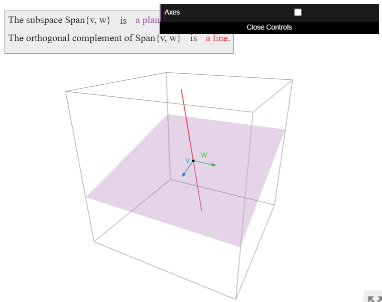
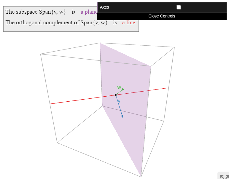
Ортогональним доповненням площини$\color{blue}W$ в$\mathbb{R}^3$ є перпендикулярна лінія$\color{Green}W^\perp$.

Малюнок$\PageIndex{5}$

Приклад$\PageIndex{3}$: Interactive: Orthogonal complements in $\mathbb{R}^3$

Малюнок$\PageIndex{6}$: The orthogonal complement of the plane spanned by $v,w$ is the perpendicular line. Click and drag the heads of $v,w$ to change the plane.

We see in the above pictures that $(W^\perp)^\perp = W$.

Example $\PageIndex{4}$

The orthogonal complement of $\mathbb{R}^n$ is $\{0\}\text{,}$ since the zero vector is the only vector that is orthogonal to all of the vectors in $\mathbb{R}^n$.

For the same reason, we have $\{0\}^\perp = \mathbb{R}^n$.

Computing Orthogonal Complements

Since any subspace is a span, the following proposition gives a recipe for computing the orthogonal complement of any subspace. However, below we will give several shortcuts for computing the orthogonal complements of other common kinds of subspaces–in particular, null spaces. To compute the orthogonal complement of a general subspace, usually it is best to rewrite the subspace as the column space or null space of a matrix, as in Note 2.6.3 in Section 2.6.

Proposition $\PageIndex{1}$: The Orthogonal Complement of a Column Space

Let $A$ be a matrix and let $W=\text{Col}(A)$. Then

$$W^\perp = \text{Nul}(A^T). \nonumber$$

Proof

To justify the first equality, we need to show that a vector $x$ is perpendicular to the all of the vectors in $W$ if and only if it is perpendicular only to $v_1,v_2,\ldots,v_m$. Since the $v_i$ are contained in $W\text{,}$ we really only have to show that if $x\cdot v_1 = x\cdot v_2 = \cdots = x\cdot v_m = 0\text{,}$ then $x$ is perpendicular to every vector $v$ in $W$. Indeed, any vector in $W$ has the form $v = c_1v_1 + c_2v_2 + \cdots + c_mv_m$ for suitable scalars $c_1,c_2,\ldots,c_m\text{,}$ so

$$\begin{split} x\cdot v \amp= x\cdot(c_1v_1 + c_2v_2 + \cdots + c_mv_m) \\ \amp= c_1(x\cdot v_1) + c_2(x\cdot v_2) + \cdots + c_m(x\cdot v_m) \\ \amp= c_1(0) + c_2(0) + \cdots + c_m(0) = 0. \end{split} \nonumber$$

Therefore, $x$ is in $W^\perp.$

To prove the second equality, we let

$$A = \left(\begin{array}{c}—v_1^T— \\ —v_2^T— \\ \vdots \\ —v_m^T—\end{array}\right). \nonumber$$

By the row-column rule for matrix multiplication Definition 2.3.3 in Section 2.3, for any vector $x$ in $\mathbb{R}^n$ we have

$$Ax = \left(\begin{array}{c}v_1^Tx \\ v_2^Tx\\ \vdots\\ v_m^Tx\end{array}\right) = \left(\begin{array}{c}v_1\cdot x\\ v_2\cdot x\\ \vdots \\ v_m\cdot x\end{array}\right). \nonumber$$

Therefore, $x$ is in $\text{Nul}(A)$ if and only if $x$ is perpendicular to each vector $v_1,v_2,\ldots,v_m$.

Since column spaces are the same as spans, we can rephrase the proposition as follows. Let $v_1,v_2,\ldots,v_m$ be vectors in $\mathbb{R}^n \text{,}$ and let $W = \text{Span}\{v_1,v_2,\ldots,v_m\}$. Then

$$W^\perp = \bigl\{\text{all vectors orthogonal to each $v_1,v_2,\ldots,v_m$}\bigr\} = \text{Nul}\left(\begin{array}{c}—v_1^T— \\ —v_2^T— \\ \vdots \\ —v_m^T—\end{array}\right). \nonumber$$

Again, it is important to be able to go easily back and forth between spans and column spaces. If you are handed a span, you can apply the proposition once you have rewritten your span as a column space.

By the proposition, computing the orthogonal complement of a span means solving a system of linear equations. For example, if

$$v_1 = \left(\begin{array}{c}1\\7\\2\end{array}\right) \qquad v_2 = \left(\begin{array}{c}-2\\3\\1\end{array}\right) \nonumber$$

then $\text{Span}\{v_1,v_2\}^\perp$ is the solution set of the homogeneous linear system associated to the matrix

$$\left(\begin{array}{c}—v_1^T— \\ —v_2^T—\end{array}\right) = \left(\begin{array}{ccc}1&7&2\\-2&3&1\end{array}\right). \nonumber$$

This is the solution set of the system of equations

$$\left\{\begin{array}{rrrrrrr}x_1 &+& 7x_2 &+& 2x_3 &=& 0\\ -2x_1 &+& 3x_2 &+& x_3 &=&0.\end{array}\right.\nonumber$$

Example $\PageIndex{5}$

Compute $W^\perp\text{,}$ where

$$W = \text{Span}\left\{\left(\begin{array}{c}1\\7\\2\end{array}\right),\;\left(\begin{array}{c}-2\\3\\1\end{array}\right)\right\}. \nonumber$$

Solution

According to Proposition $\PageIndex{1}$, we need to compute the null space of the matrix

$$\left(\begin{array}{ccc}1&7&2\\-2&3&1\end{array}\right) \;\xrightarrow{\text{RREF}}\; \left(\begin{array}{ccc}1&0&-1/17 \\ 0&1&5/17\end{array}\right). \nonumber$$

The free variable is $x_3\text{,}$ so the parametric form of the solution set is $x_1=x_3/17,\,x_2=-5x_3/17\text{,}$ and the parametric vector form is

$$\left(\begin{array}{c}x_1\\x_2\\x_3\end{array}\right) = x_3\left(\begin{array}{c}1/17 \\ -5/17\\1\end{array}\right). \nonumber$$

Scaling by a factor of $17\text{,}$ we see that

$$W^\perp = \text{Span}\left\{\left(\begin{array}{c}1\\-5\\17\end{array}\right)\right\}. \nonumber$$

We can check our work:

$$\left(\begin{array}{c}1\\7\\2\end{array}\right)\cdot\left(\begin{array}{c}1\\-5\\17\end{array}\right) = 0 \qquad \left(\begin{array}{c}-2\\3\\1\end{array}\right)\cdot\left(\begin{array}{c}1\\-5\\17\end{array}\right) = 0. \nonumber$$

Example $\PageIndex{6}$

Find all vectors orthogonal to $v = \left(\begin{array}{c}1\\1\\-1\end{array}\right).$

Solution

According to Proposition $\PageIndex{1}$, we need to compute the null space of the matrix

$$A = \left(\begin{array}{c}—v—\end{array}\right) = \left(\begin{array}{ccc}1&1&-1\end{array}\right). \nonumber$$

This matrix is in reduced-row echelon form. The parametric form for the solution set is $x_1 = -x_2 + x_3\text{,}$ so the parametric vector form of the general solution is

$$x = \left(\begin{array}{c}x_1\\x_2\\x_3\end{array}\right) = x_2\left(\begin{array}{c}-1\\1\\0\end{array}\right) + x_3\left(\begin{array}{c}1\\0\\1\end{array}\right). \nonumber$$

Therefore, the answer is the plane

$$\text{Span}\left\{\left(\begin{array}{c}-1\\1\\0\end{array}\right),\;\left(\begin{array}{c}1\\0\\1\end{array}\right)\right\}. \nonumber$$

Figure $\PageIndex{7}$: The set of all vectors perpendicular to $v$.

Example $\PageIndex{7}$

Compute

$$\text{Span}\left\{\left(\begin{array}{c}1\\1\\-1\end{array}\right),\;\left(\begin{array}{c}1\\1\\1\end{array}\right)\right\}^\perp. \nonumber$$

Solution

According to Proposition $\PageIndex{1}$, we need to compute the null space of the matrix

$$A = \left(\begin{array}{ccc}1&1&-1\\1&1&1\end{array}\right)\;\xrightarrow{\text{RREF}}\;\left(\begin{array}{ccc}1&1&0\\0&0&1\end{array}\right). \nonumber$$

The parametric vector form of the solution is

$$\left(\begin{array}{c}x_1\\x_2\\x_3\end{array}\right) = x_2\left(\begin{array}{c}-1\\1\\0\end{array}\right). \nonumber$$

Therefore, the answer is the line

$$\text{Span}\left\{\left(\begin{array}{c}-1\\1\\0\end{array}\right)\right\}. \nonumber$$

Figure $\PageIndex{8}$: The orthogonal complement of the plane spanned by $v = (1,1,-1)$ and $w = (1, 1, 1)$.

In order to find shortcuts for computing orthogonal complements, we need the following basic facts. Looking back the the above examples, all of these facts should be believable.

Fact $\PageIndex{1}$: Facts about Orthogonal Complements

Let $W$ be a subspace of $\mathbb{R}^n$. Then:

1. $W^\perp$ is also a subspace of $\mathbb{R}^n .$
2. $(W^\perp)^\perp = W.$
3. $\dim(W) + \dim(W^\perp) = n.$

Proof

For the first assertion, we verify the three defining properties of subspaces, Definition 2.6.2 in Section 2.6.

1. The zero vector is in $W^\perp$ because the zero vector is orthogonal to every vector in $\mathbb{R}^n$.
2. Let $u,v$ be in $W^\perp\text{,}$ so $u\cdot x = 0$ and $v\cdot x = 0$ for every vector $x$ in $W$. We must verify that $(u+v)\cdot x = 0$ for every $x$ in $W$. Indeed, we have $$(u+v)\cdot x = u\cdot x + v\cdot x = 0 + 0 = 0. \nonumber$$
3. Let $u$ be in $W^\perp\text{,}$ so $u\cdot x = 0$ for every $x$ in $W\text{,}$ and let $c$ be a scalar. We must verify that $(cu)\cdot x = 0$ for every $x$ in $W$. Indeed, we have $$(cu)\cdot x = c(u\cdot x) = c0 = 0. \nonumber$$

Next we prove the third assertion. Let $v_1,v_2,\ldots,v_m$ be a basis for $W\text{,}$ so $m = \dim(W)\text{,}$ and let $v_{m+1},v_{m+2},\ldots,v_k$ be a basis for $W^\perp\text{,}$ so $k-m = \dim(W^\perp)$. We need to show $k=n$. First we claim that $\{v_1,v_2,\ldots,v_m,v_{m+1},v_{m+2},\ldots,v_k\}$ is linearly independent. Suppose that $c_1v_1 + c_2v_2 + \cdots + c_kv_k = 0$. Let $w = c_1v_1 + c_2v_2 + \cdots + c_mv_m$ and $w' = c_{m+1}v_{m+1} + c_{m+2}v_{m+2} + \cdots + c_kv_k\text{,}$ so $w$ is in $W\text{,}$ $w'$ is in $W'\text{,}$ and $w + w' = 0$. Then $w = -w'$ is in both $W$ and $W^\perp\text{,}$ which implies $w$ is perpendicular to itself. In particular, $w\cdot w = 0\text{,}$ so $w = 0\text{,}$ and hence $w' = 0$. Therefore, all coefficients $c_i$ are equal to zero, because $\{v_1,v_2,\ldots,v_m\}$ and $\{v_{m+1},v_{m+2},\ldots,v_k\}$ are linearly independent.

It follows from the previous paragraph that $k \leq n$. Suppose that $k \lt n$. Then the matrix

$$A = \left(\begin{array}{c}—v_1^T— \\ —v_2^T— \\ \vdots \\ —v_k^T—\end{array}\right) \nonumber$$

has more columns than rows (it is “wide”), so its null space is nonzero by Note 3.2.1 in Section 3.2. Let $x$ be a nonzero vector in $\text{Nul}(A)$. Then

$$0 = Ax = \left(\begin{array}{c}v_1^Tx \\ v_2^Tx \\ \vdots \\ v_k^Tx\end{array}\right) = \left(\begin{array}{c}v_1\cdot x\\ v_2\cdot x\\ \vdots \\ v_k\cdot x\end{array}\right) \nonumber$$

by the row-column rule for matrix multiplication Definition 2.3.3 in Section 2.3. Since $v_1\cdot x = v_2\cdot x = \cdots = v_m\cdot x = 0\text{,}$ it follows from Proposition $\PageIndex{1}$ that $x$ is in $W^\perp\text{,}$ and similarly, $x$ is in $(W^\perp)^\perp$. As above, this implies $x$ is orthogonal to itself, which contradicts our assumption that $x$ is nonzero. Therefore, $k = n\text{,}$ as desired.

Finally, we prove the second assertion. Clearly $W$ is contained in $(W^\perp)^\perp\text{:}$ this says that everything in $W$ is perpendicular to the set of all vectors perpendicular to everything in $W$. Let $m=\dim(W).$ By 3, we have $\dim(W^\perp) = n-m\text{,}$ so $\dim((W^\perp)^\perp) = n - (n-m) = m$. The only $m$-dimensional subspace of $(W^\perp)^\perp$ is all of $(W^\perp)^\perp\text{,}$ so $(W^\perp)^\perp = W.$

See subsection Pictures of orthogonal complements, for pictures of the second property. As for the third: for example, if $W$ is a ($2$-dimensional) plane in $\mathbb{R}^4\text{,}$ then $W^\perp$ is another ($2$-dimensional) plane. Explicitly, we have

$$\begin{aligned}\text{Span}\{e_1,e_2\}^{\perp}&=\left\{\left(\begin{array}{c}x\\y\\z\\w\end{array}\right)\text{ in }\mathbb{R}\left| \left(\begin{array}{c}x\\y\\z\\w\end{array}\right)\cdot\left(\begin{array}{c}1\\0\\0\\0\end{array}\right)=0\text{ and }\left(\begin{array}{c}x\\y\\z\\w\end{array}\right)\left(\begin{array}{c}0\\1\\0\\0\end{array}\right)=0\right.\right\} \\ &=\left\{\left(\begin{array}{c}0\\0\\z\\w\end{array}\right)\text{ in }\mathbb{R}^4\right\}=\text{Span}\{e_3,e_4\}:\end{aligned}$$

the orthogonal complement of the $xy$-plane is the $zw$-plane.

Definition $\PageIndex{2}$: Row Space

The row space of a matrix $A$ is the span of the rows of $A\text{,}$ and is denoted $\text{Row}(A)$.

If $A$ is an $m\times n$ matrix, then the rows of $A$ are vectors with $n$ entries, so $\text{Row}(A)$ is a subspace of $\mathbb{R}^n$. Equivalently, since the rows of $A$ are the columns of $A^T\text{,}$ the row space of $A$ is the column space of $A^T\text{:}$

$$\text{Row}(A) = \text{Col}(A^T). \nonumber$$

We showed in the above Proposition $\PageIndex{3}$ that if $A$ has rows $v_1^T,v_2^T,\ldots,v_m^T\text{,}$ then

$$\text{Row}(A)^\perp = \text{Span}\{v_1,v_2,\ldots,v_m\}^\perp = \text{Nul}(A). \nonumber$$

Taking orthogonal complements of both sides and using the second fact $\PageIndex{1}$ gives

$$\text{Row}(A) = \text{Nul}(A)^\perp. \nonumber$$

Replacing $A$ by $A^T$ and remembering that $\text{Row}(A)=\text{Col}(A^T)$ gives

$$\text{Col}(A)^\perp = \text{Nul}(A^T) \quad\text{and}\quad \text{Col}(A) = \text{Nul}(A^T)^\perp. \nonumber$$

To summarize:

Recipe: Shortcuts for Computing Orthogonal Complements

For any vectors $v_1,v_2,\ldots,v_m\text{,}$ we have

$$\text{Span}\{v_1,v_2,\ldots,v_m\}^\perp = \text{Nul}\left(\begin{array}{c}—v_1^T— \\ —v_2^T— \\ \vdots \\ —v_m^T—\end{array}\right) . \nonumber$$

For any matrix $A\text{,}$ we have

$$\begin{aligned} \text{Row}(A)^\perp &= \text{Nul}(A) & \text{Nul}(A)^\perp &= \text{Row}(A) \\ \text{Col}(A)^\perp &= \text{Nul}(A^T)\quad & \text{Nul}(A^T)^\perp &= \text{Col}(A). \end{aligned} \nonumber$$

As mentioned in the beginning of this subsection, in order to compute the orthogonal complement of a general subspace, usually it is best to rewrite the subspace as the column space or null space of a matrix.

Example $\PageIndex{8}$: Orthogonal complement of a subspace

Compute the orthogonal complement of the subspace

$$W = \bigl\{(x,y,z) \text{ in } \mathbb{R}^3 \mid 3x + 2y = z\bigr\}. \nonumber$$

Solution

Rewriting, we see that $W$ is the solution set of the system of equations $3x + 2y - z = 0\text{,}$ i.e., the null space of the matrix $A = \left(\begin{array}{ccc}3&2&-1\end{array}\right).$ Therefore,

$$W^\perp = \text{Row}(A) = \text{Span}\left\{\left(\begin{array}{c}3\\2\\-1\end{array}\right)\right\}. \nonumber$$

No row reduction was needed!

Example $\PageIndex{9}$: Orthogonal complement of an eigenspace

Find the orthogonal complement of the $5$-eigenspace of the matrix

$$A=\left(\begin{array}{ccc}2&4&-1\\3&2&0\\-2&4&3\end{array}\right).\nonumber$$

Solution

The $5$-eigenspace is

$$W = \text{Nul}(A - 5I_3) = \text{Nul}\left(\begin{array}{ccc}-3&4&-1\\3&-3&0\\-2&4&-2\end{array}\right), \nonumber$$

so

$$W^\perp = \text{Row}\left(\begin{array}{ccc}-3&4&-1\\3&-3&0\\-2&4&-2\end{array}\right) = \text{Span}\left\{\left(\begin{array}{c}-3\\4\\-1\end{array}\right),\;\left(\begin{array}{c}3\\-3\\0\end{array}\right),\;\left(\begin{array}{c}-2\\4\\-2\end{array}\right)\right\}. \nonumber$$

These vectors are necessarily linearly dependent (why)?

Row rank and Column Rank

Suppose that $A$ is an $m \times n$ matrix. Let us refer to the dimensions of $\text{Col}(A)$ and $\text{Row}(A)$ as the row rank and the column rank of $A$ (note that the column rank of $A$ is the same as the rank of $A$). The next theorem says that the row and column ranks are the same. This is surprising for a couple of reasons. First, $\text{Row}(A)$ lies in $\mathbb{R}^n$ and $\text{Col}(A)$ lies in $\mathbb{R}^m$. Also, the theorem implies that $A$ and $A^T$ have the same number of pivots, even though the reduced row echelon forms of $A$ and $A^T$ have nothing to do with each other otherwise.

Theorem $\PageIndex{1}$

Let $A$ be a matrix. Then the row rank of $A$ is equal to the column rank of $A$.

Proof

By Theorem 2.9.1 in Section 2.9, we have

$$\dim\text{Col}(A) + \dim\text{Nul}(A) = n. \nonumber$$

On the other hand the third fact $\PageIndex{1}$ says that

$$\dim\text{Nul}(A)^\perp + \dim\text{Nul}(A) = n, \nonumber$$

which implies $\dim\text{Col}(A) = \dim\text{Nul}(A)^\perp$. Since $\text{Nul}(A)^\perp = \text{Row}(A),$ we have

$$\dim\text{Col}(A) = \dim\text{Row}(A)\text{,} \nonumber$$

as desired.

In particular, by Corollary 2.7.1 in Section 2.7 both the row rank and the column rank are equal to the number of pivots of $A$.