1.8: флюс
- Page ID
- 78595

Добутком напруженості електричного поля і площі є потік\(\Phi_E\). Whereas \(E\) is an intensive quantity, \(\Phi_E\) is an extensive quantity. It dimensions are ML3T-2Q-1 and its SI units are N m2 C-1, although later on, after we have met the unit called the volt, we shall prefer to express \(\Phi_E\) in V m.
Зі збільшенням ступенів витонченості флюс може бути визначено математично як:
\[\Phi_E = EA\]
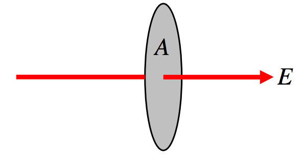
\(\text{FIGURE I.4}\): Потік, який перпендикулярний поверхні.
\[\Phi_E = EA \cos \theta = \textbf{E} \cdot \textbf{A} \]
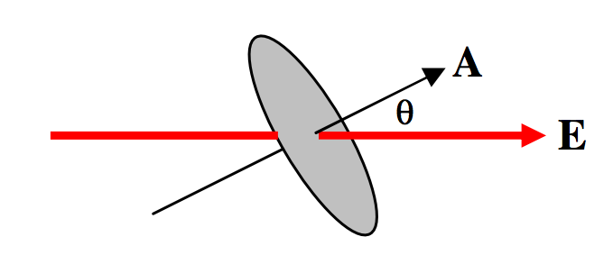
\(\text{FIGURE I.5}\): Flow that is at an angle to the surface.
Зверніть увагу, що\(\textbf{E}\) is a vector, but \(\Phi_E\) is a scalar.
\[\Phi_E = \iint \textbf{E} \cdot d\textbf{A} \]
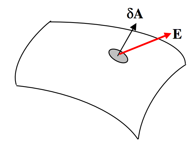
\(\text{FIGURE I.6}\)
Ми також можемо визначити\(D\)-flux by
\[\Phi_D=\iint \textbf{D}\cdot d\textbf{A}.\]
Розміри\(\Phi_D\) are just \(Q\) and the SI units are coulombs (C).
Приклад по порядку:
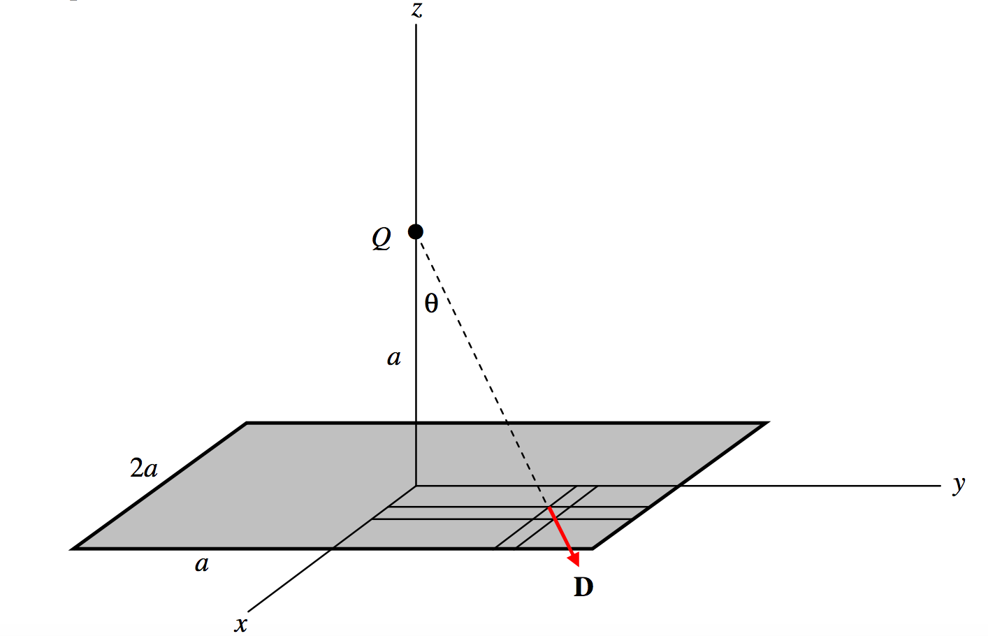
\(\text{FIGURE I.7}\)
Розглянемо квадрат сторони\(2a\) in the xy-plane as shown. Suppose there is a positive charge \(Q\) at a height \(a\) on the \(z\)-axis. Calculate the total \(D\)-flux, \(\Phi_D\) through the area.
Розглянемо стихійну область\(dxdy\) at (\(x,\, y ,\, 0\)). Its distance from \(Q\) is \((a^2+x^2+y^2)^{1/2}\) so the magnitude of the \(D\)-field there is \(\frac{Q}{4\pi}\cdot \frac{1}{a^2+x^2+y^2}\). The scalar product of this with the area is \(\frac{Q}{4\pi}\cdot \frac{1}{a^2+x^2+y^2}\cdot \cos \theta dxdy,\text{ and }\cos \theta = \frac{a}{(a^2+x^2+y^2)^{1/2}}\). The surface integral of \(\textbf{D}\) over the whole area is
\[\label{1.8.1}\iint D\cdot dA=\frac{Qa}{\pi}\int_0^a \int_0^a \frac{dxdy}{(a^2+x^2+y^2)^{3/2}}.\]
Тепер все, що нам потрібно зробити, це хороший і легкий інтеграл. Нехай\(x=\sqrt{a^2+y^2}\tan ψ\) and the inner integral \(\int_0^a \frac{dx}{(a^2+x^2+y^2)^{3/2}}\) reduces, after some modest algebra, to \(\frac{a}{(a^2+y^2)\sqrt{2a^2+y^2}}\). Thus we now have
\[\label{1.8.2}\iint D\cdot dA = \frac{Qa^2}{\pi}\int_0^a \frac{dy}{(a^2+y^2)\sqrt{2a^2+y^2}}.\]
З подальшою заміною\(a^2+y^2=a^2 \sec \omega\) this reduces, after more careful algebra, to
\[\iint D\cdot dA=\frac{Q}{6}.\label{1.8.3}\]
Два додаткових приклади обчислення поверхневих інтегралів можна знайти в розділі 5.6 розділу «Небесна механіка» цих приміток. Вони мають справу з гравітаційними полями, але вони по суті такі ж, як електростатичний випадок; просто замінити\(Q\) for m and -1/(4\(\pi \epsilon\)) for \(G\).
Я закликаю читачів насправді пройти через біль і алгебру та тригонометрію цих трьох прикладів, щоб вони могли оцінити тим більше, у наступному розділі, силу теореми Гаусса.