4.5: Моделі погіршення штучної нейронної мережі
- Page ID
- 8786

Штучні нейронні мережі можуть служити альтернативою регресійним або марківським моделям погіршення. Вони засновані на аналогії з тим, як поводяться прості біологічні мізки при передачі сигналів між окремими нервовими клітинами. Вони виникли в роботі над штучним інтелектом і машинним навчанням.
Малюнок 4.5.1 ілюструє нейронну мережу. Входами можуть бути значення індексу стану, вік або погодні ефекти. Виходами можуть бути ймовірності переходу до певних умов протягом року. Малюнок 4.5.1 ілюструє обробку сигналу, яка відбуватиметься всередині кожного зі штучних нейронів (представлена у вигляді кіл на малюнку 4.5.1). Вхідні сигнали зважуються, комбінуються і перетворюються в вихідну активацію.
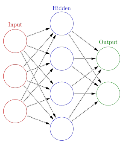
Малюнок\(\PageIndex{1}\): Illustration of a Neural Network with Input, Hidden and Output Stages. Source: By Glosser.ca - Own work, Derivative of File:Artificial neural network.svg, CC BY-SA 3.0, https://commons.wikimedia.org/w/inde...curid=24913461.
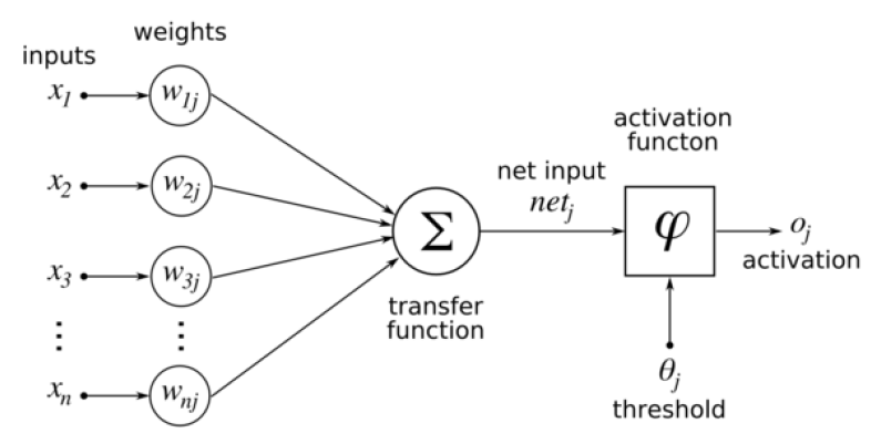
Artificial neural networks are typically ‘trained’ with a learning set. For a deterioration model, inputs might consist of conditions (and other relevant factors) in the base year and the training outputs would be the observed conditions in the following year. Training consists of altering parameters (such as the weights in Figure 4.5.2) to best reproduce the results observed in the training set.
Artificial neural networks are not frequently used for component deterioration modelling. One drawback to their use is the ‘black box’ nature of the results where the various weights and activation functions are difficult to interpret (or even obtain). Also, artificial neural networks typically have many more parameters than other types of models, requiring more data to be robust.
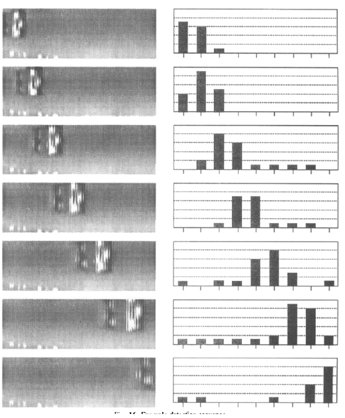
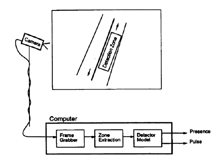
Infrastructure managers are more likely to encounter artificial neural networks in conjunction with sensor interpretation. For example, artificial neural networks can be used to identify vehicles or pavement distress from video inputs. Figure 4.5.3 illustrates a video-based system for vehicle identification. A frame from the camera is divided into a two dimensional set of tiles within a pre-defined detection zone and the color and brightness of the pixels within each tile are input to an artificial neural network vehicle detector model. A training set of images with and without vehicles is used to adjust parameters in the detector model. In turn, traffic identification of this type can be used in a deterioration model for pavement condition.
A detection sequence for the video vehicle identification is illustrated in Figure 4.5.4. As the vehicle moves through the detection zone, counting output is activated for each part of the zone.